Draw a Great Circle Line

Flight or sailing road along the shortest path betwixt 2 points on a globe'southward surface

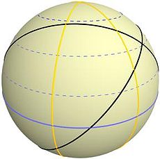
Orthodromic course drawn on the globe globe.

Great-circle navigation or orthodromic navigation (related to orthodromic course; from the Greek ορθóς, right bending, and δρóμος, path) is the exercise of navigating a vessel (a transport or aircraft) along a keen circle. Such routes yield the shortest distance between two points on the globe.^[i]

Course [edit]

Figure 1. The slap-up circle path betwixt (φ₁, λ_ane) and (φ₂, λ_ii).

The great circle path may be institute using spherical trigonometry; this is the spherical version of the inverse geodetic problem. If a navigator begins at P _i = (φ_i,λ₁) and plans to travel the great circle to a point at point P _ii = (φ₂,λ_two) (see Fig. 1, φ is the latitude, positive due north, and λ is the longitude, positive e), the initial and final courses α₁ and α_two are given past formulas for solving a spherical triangle

${\displaystyle {\brainstorm{aligned}\tan \blastoff _{1}&={\frac {\cos \phi _{2}\sin \lambda _{12}}{\cos \phi _{1}\sin \phi _{2}-\sin \phi _{1}\cos \phi _{2}\cos \lambda _{12}}},\\\tan \alpha _{two}&={\frac {\cos \phi _{1}\sin \lambda _{12}}{-\cos \phi _{2}\sin \phi _{ane}+\sin \phi _{2}\cos \phi _{1}\cos \lambda _{12}}},\\\cease{aligned}}}$

where λ₁₂ = λ₂ − λ₁ ^{[notation 1]} and the quadrants of α₁,α₂ are determined by the signs of the numerator and denominator in the tangent formulas (e.g., using the atan2 office). The central angle between the two points, σ₁₂, is given by

${\displaystyle \tan \sigma _{12}={\frac {\sqrt {(\cos \phi _{ane}\sin \phi _{2}-\sin \phi _{1}\cos \phi _{2}\cos \lambda _{12})^{2}+(\cos \phi _{2}\sin \lambda _{12})^{2}}}{\sin \phi _{1}\sin \phi _{2}+\cos \phi _{1}\cos \phi _{2}\cos \lambda _{12}}}.}$ ^{[note ii] [note 3]}

(The numerator of this formula contains the quantities that were used to decide tanα₁.) The distance along the bang-up circle volition then be s ₁₂ =Rσ₁₂, where R is the assumed radius of the world and σ₁₂ is expressed in radians. Using the mean earth radius, R =R ₁ ≈ 6,371 km (3,959 mi) yields results for the distance southward ₁₂ which are within 1% of the geodesic length for the WGS84 ellipsoid; see Geodesics on an ellipsoid for details.

Finding way-points [edit]

To find the style-points, that is the positions of selected points on the great circle between P ₁ and P ₂, we outset extrapolate the dandy circle back to its node A, the point at which the great circle crosses the equator in the northward management: let the longitude of this indicate exist λ₀ — see Fig 1. The azimuth at this point, α₀, is given past

${\displaystyle \tan \blastoff _{0}={\frac {\sin \alpha _{1}\cos \phi _{1}}{\sqrt {\cos ^{2}\alpha _{ane}+\sin ^{2}\blastoff _{1}\sin ^{2}\phi _{1}}}}.}$ ^{[note 4]}

Let the angular distances along the peachy circle from A to P ₁ and P ₂ be σ₀₁ and σ₀₂ respectively. Then using Napier's rules nosotros accept

${\displaystyle \tan \sigma _{01}={\frac {\tan \phi _{1}}{\cos \alpha _{1}}}\qquad }$ (If φ_ane = 0 and α_ane = 1⁄2 π, use σ₀₁ = 0).

This gives σ₀₁, whence σ₀₂ = σ₀₁ + σ₁₂.

The longitude at the node is plant from

${\displaystyle {\begin{aligned}\tan \lambda _{01}&={\frac {\sin \blastoff _{0}\sin \sigma _{01}}{\cos \sigma _{01}}},\\\lambda _{0}&=\lambda _{1}-\lambda _{01}.\end{aligned}}}$

Effigy ii. The not bad circle path between a node (an equator crossing) and an arbitrary point (φ,λ).

Finally, calculate the position and azimuth at an arbitrary bespeak, P (see Fig. 2), by the spherical version of the direct geodesic problem.^{[note 5]} Napier'south rules requite

${\displaystyle {\colour {white}.\,\qquad )}\tan \phi ={\frac {\cos \alpha _{0}\sin \sigma }{\sqrt {\cos ^{2}\sigma +\sin ^{2}\alpha _{0}\sin ^{2}\sigma }}},}$ ^{[note 6]}

${\displaystyle {\begin{aligned}\tan(\lambda -\lambda _{0})&={\frac {\sin \alpha _{0}\sin \sigma }{\cos \sigma }},\\\tan \alpha &={\frac {\tan \alpha _{0}}{\cos \sigma }}.\end{aligned}}}$

The atan2 function should exist used to determine σ₀₁, λ, and α. For example, to discover the midpoint of the path, substitute σ = 1⁄ii (σ₀₁ + σ₀₂); alternatively to find the bespeak a distance d from the starting point, take σ = σ₀₁ +d/R. Likewise, the vertex, the betoken on the dandy circumvolve with greatest latitude, is found by substituting σ = + 1⁄2 π. It may be convenient to parameterize the route in terms of the longitude using

${\displaystyle \tan \phi =\cot \alpha _{0}\sin(\lambda -\lambda _{0}).}$ ^{[note seven]}

Latitudes at regular intervals of longitude tin can be found and the resulting positions transferred to the Mercator nautical chart allowing the great circle to be approximated by a series of rhumb lines. The path determined in this mode gives the great ellipse joining the terminate points, provided the coordinates ${\displaystyle (\phi ,\lambda )}$ are interpreted as geographic coordinates on the ellipsoid.

These formulas utilize to a spherical model of the earth. They are also used in solving for the great circumvolve on the auxiliary sphere which is a device for finding the shortest path, or geodesic, on an ellipsoid of revolution; encounter the commodity on geodesics on an ellipsoid.

Example [edit]

Compute the great circumvolve route from Valparaíso, φ₁ = −33°, λ_one = −71.vi°, to Shanghai, φ₂ = 31.4°, λ_two = 121.8°.

The formulas for course and distance give λ₁₂ = −166.6°,^{[note 8]} α₁ = −94.41°, α_ii = −78.42°, and σ₁₂ = 168.56°. Taking the earth radius to be R = 6371 km, the altitude is s ₁₂ = 18743 km.

To compute points along the route, first detect α₀ = −56.74°, σ₁ = −96.76°, σ_two = 71.8°, λ₀₁ = 98.07°, and λ₀ = −169.67°. And so to compute the midpoint of the road (for example), take σ = 1⁄2 (σ₁ + σ_two) = −12.48°, and solve for φ = −6.81°, λ = −159.xviii°, and α = −57.36°.

If the geodesic is computed accurately on the WGS84 ellipsoid,^[iv] the results are α_i = −94.82°, α_two = −78.29°, and south ₁₂ = 18752 km. The midpoint of the geodesic is φ = −7.07°, λ = −159.31°, α = −57.45°.

Gnomonic chart [edit]

A directly line drawn on a gnomonic chart would be a great circle rail. When this is transferred to a Mercator chart, it becomes a curve. The positions are transferred at a convenient interval of longitude and this is plotted on the Mercator chart.

See likewise [edit]

• Compass rose
• Bully circle
• Bully-circle distance
• Swell ellipse
• Geodesics on an ellipsoid
• Geographical distance
• Isoazimuthal
• Loxodromic navigation
• Map
  • Portolan map
• Marine sandglass
• Rhumb line
• Spherical trigonometry
• Windrose network

Notes [edit]

1. ^ In the article on groovy-circle distances, the notation Δλ = λ₁₂ and Δσ = σ₁₂ is used. The notation in this commodity is needed to deal with differences between other points, e.1000., λ₀₁.
2. ^ A simpler formula is

   ${\displaystyle \cos \sigma _{12}=\sin \phi _{1}\sin \phi _{2}+\cos \phi _{1}\cos \phi _{ii}\cos \lambda _{12};}$

   notwithstanding, this is less accurate if σ₁₂ small.
3. ^ These equations for α_one,α₂,σ₁₂ are suitable for implementation on modern calculators and computers. For hand computations with logarithms, Delambre's analogies^[two] were usually used:

   ${\displaystyle {\brainstorm{aligned}\cos {\tfrac {1}{two}}(\alpha _{2}+\blastoff _{one})\sin {\tfrac {ane}{2}}\sigma _{12}&=\sin {\tfrac {ane}{2}}(\phi _{2}-\phi _{ane})\cos {\tfrac {1}{2}}\lambda _{12},\\\sin {\tfrac {1}{2}}(\alpha _{two}+\alpha _{1})\sin {\tfrac {1}{2}}\sigma _{12}&=\cos {\tfrac {1}{2}}(\phi _{2}+\phi _{1})\sin {\tfrac {1}{2}}\lambda _{12},\\\cos {\tfrac {1}{2}}(\blastoff _{2}-\alpha _{ane})\cos {\tfrac {one}{ii}}\sigma _{12}&=\cos {\tfrac {1}{two}}(\phi _{two}-\phi _{one})\cos {\tfrac {1}{2}}\lambda _{12},\\\sin {\tfrac {1}{2}}(\blastoff _{ii}-\alpha _{1})\cos {\tfrac {i}{ii}}\sigma _{12}&=\sin {\tfrac {1}{2}}(\phi _{2}+\phi _{1})\sin {\tfrac {one}{two}}\lambda _{12}.\terminate{aligned}}}$

   McCaw^[3] refers to these equations as being in "logarithmic class", by which he means that all the trigonometric terms appear as products; this minimizes the number of table lookups required. Furthermore, the back-up in these formulas serves as a check in hand calculations. If using these equations to determine the shorter path on the great circle, it is necessary to ensure that |λ₁₂| ≤ π (otherwise the longer path is plant).
4. ^ A simpler formula is

   ${\displaystyle \sin \alpha _{0}=\sin \alpha _{1}\cos \phi _{1};}$

   withal, this is less authentic α₀ ≈ ± 1⁄two π.
5. ^ The direct geodesic problem, finding the position of P _two given P ₁, α₁, and southward ₁₂, can also be solved by formulas for solving a spherical triangle, as follows,

   ${\displaystyle {\begin{aligned}\sigma _{12}&=s_{12}/R,\\\sin \phi _{2}&=\sin \phi _{1}\cos \sigma _{12}+\cos \phi _{i}\sin \sigma _{12}\cos \alpha _{1},\quad {\text{or}}\\\tan \phi _{2}&={\frac {\sin \phi _{i}\cos \sigma _{12}+\cos \phi _{1}\sin \sigma _{12}\cos \alpha _{one}}{\sqrt {(\cos \phi _{i}\cos \sigma _{12}-\sin \phi _{1}\sin \sigma _{12}\cos \blastoff _{1})^{2}+(\sin \sigma _{12}\sin \alpha _{ane})^{2}}}},\\\tan \lambda _{12}&={\frac {\sin \sigma _{12}\sin \blastoff _{one}}{\cos \phi _{1}\cos \sigma _{12}-\sin \phi _{ane}\sin \sigma _{12}\cos \alpha _{1}}},\\\lambda _{ii}&=\lambda _{1}+\lambda _{12},\\\tan \blastoff _{ii}&={\frac {\sin \alpha _{1}}{\cos \sigma _{12}\cos \alpha _{one}-\tan \phi _{1}\sin \sigma _{12}}}.\end{aligned}}}$

   The solution for way-points given in the principal text is more general than this solution in that it allows mode-points at specified longitudes to be found. In addition, the solution for σ (i.east., the position of the node) is needed when finding geodesics on an ellipsoid by means of the auxiliary sphere.
6. ^ A simpler formula is

   ${\displaystyle \sin \phi =\cos \alpha _{0}\sin \sigma ;}$

   however, this is less authentic when φ ≈ ± one⁄2 π
7. ^ The post-obit is used: ${\displaystyle \cos \sigma =\cos \phi \cos(\lambda -\lambda _{0})}$
8. ^ λ₁₂ is reduced to the range [−180°, 180°] by adding or subtracting 360° every bit necessary

References [edit]

1. ^ Adam Weintrit; Tomasz Neumann (7 June 2011). Methods and Algorithms in Navigation: Marine Navigation and Condom of Bounding main Transportation. CRC Press. pp. 139–. ISBN978-0-415-69114-7.
2. ^ Todhunter, I. (1871). Spherical Trigonometry (third ed.). MacMillan. p. 26.
3. ^ McCaw, K. T. (1932). "Long lines on the World". Empire Survey Review. i (6): 259–263. doi:ten.1179/sre.1932.i.vi.259.
4. ^ Karney, C. F. F. (2013). "Algorithms for geodesics". Journal of Geodesy. 87 (i): 43–55. doi:10.1007/s00190-012-0578-z.

External links [edit]

• Neat Circumvolve – from MathWorld Great Circle clarification, figures, and equations. Mathworld, Wolfram Enquiry, Inc. c1999
• Smashing Circle Mapper Interactive tool for plotting great circumvolve routes.
• Peachy Circumvolve Calculator deriving (initial) course and distance between two points.
• Groovy Circle Distance Graphical tool for drawing peachy circles over maps. Also shows distance and azimuth in a table.
• Google assist program for orthodromic navigation

funkalisome.blogspot.com

Source: https://en.wikipedia.org/wiki/Great-circle_navigation

Share this post